Changing your perspective with a change of variables

If someone asked me to summarise my memory of grade 10 maths, I would reply with a single word: Quadratics. I remember solving scores of quadratics, and by the end of the year I was pretty good at it (admittedly I was also pretty lazy, and usually just used the quadratic formula). But then I started grade 11 and my teacher threw me a curve ball with the following equation:

$e^{2x}-5e^x+4=0.$

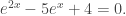
This equation is pretty intimidating the first time you see it! There’s an exponential in there so I wanted to use a logarithm, but I had no way to break up a logarithm over a sum! Of course, there is a very clean way to circumvent this. Instead of working in $x$ , we work with a new variable $y=e^x$ . Our equation is then … a quadratic!

$y^2-5y+6=0.$

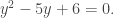
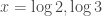
Since we can solve quadratics, we see that $y=2,3$ which gives $x=\log 2,\log 3$ .

Now, our motivating example may seem pretty insignificant. But what is interesting to me is that the general principle we used to solve it is useful, defining a new variable which is more suited to our problem and then translating the solution back to the original variable, is useful in so many situations. In fact, the reason changing variables is on my mind is because I noticed a change of variables could help me solve a problem for my honours thesis. While the solution in my honours didn’t quite pan out the way I hoped, it excited me enough to want to list some other change of variables I’ve seen throughout university.

Change of Variables in Integration

My first example is perhaps low hanging fruit. It is the change of variables formula from integral calculus: If $\varphi:[a,b]\to [\alpha,\beta]$ is a differentiable, monotone function whose derivative is continuous and $f:[\alpha,\beta]\to \mathbb{R}$ is continuous then

$\int_a^bf(\varphi(t))\varphi'(t)\, dt= \int_\alpha^\beta f(s)\, ds.$

A similar formula also holds for integrals in higher dimensions. The idea is exactly the same as in the quadratic example, the integral is easier is we choose variables that are ‘suited to the problem’.

Here is an example from the plane. Suppose we want to know the volume bounded by the paraboloid $f(x,y)=x^2+y^2+1$ and the $xy-$ plane. This is given by the integral

$\int_{\{x^2+y^\le 1\}} x^2+y^2+1\, dx\,dy,$

A rough sketch of the volume we want to calculate.

In our usual cartesian coordinates, the region $x^2+y^2\le 1$ is a little awkward to describe. Indeed, if we start with $x\in [-1,1]$ then for $(x,y)$ to be in the region we need $y^2\le 1-x^2$ so we have

$\{x^2+y^2\le 1\}= \{(x,y): -1\le x\le 1, -\sqrt{1-x^2}\le y\le \sqrt{1-x^2}\},$

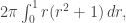
which gives the integral

$\int_{-1}^1 \int _{-\sqrt{1-x^2}}^{\sqrt{1-x^2}} x^2+y^2+1\, dy\, dx.$

Cartesian coordinates v.s. polar coordinates.

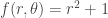
While this isn’t impossible to compute, it’s definitely not ideal. Let’s try changing variables. Rather than describing our point by its distance from the x-axis and y-axis, let describe it by its distance from the origin ( $r$ ) and its angle ( $\theta$ ) with the x-axis (i.e. use polar coordinates). Then $r^2=x^2+y^2$ , so our region is

$\{x^2+y^2\le 1\}=\{r\le 1\}$ ,

and in terms of $(r,\theta)$ we have $f(r,\theta) = r^2+1$ . In these variables, our integral becomes

$2\pi \int_0^1 r(r^2+1)\, dr,$

(the extra factor of $r$ comes from the change of variables formula, the $2\pi$ come from the angle coordinate). In either case, the value of the integral is $6\pi/4$ , but the point is that polar coordinates suit the problem better because our function and region only depend on the radial coordinate ( $r$ ), not on the angular coordinate.

Laplace’s Equation

Here is another example where polar coordinates help us solve an equation. We’ll work in the real plane again and consider the partial differential equation

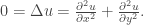
$0=\Delta u = \frac{\partial^2 u}{\partial x^2}+\frac{\partial^2 u}{\partial y^2}.$

This is called Laplace’s equation; If $u(x,y)$ gives the density of a physical quantity (e.g. heat) then Laplace’s equation expresses the fact the quantity is in equilibrium within some region.

What’s important for us to notice is that Laplace’s equation is rotation invariant. By this I mean that if $u$ solves Laplace’s equation on the plane, and if $R$ is a rotation of the plane the the function $v$ defined by first rotating the plane using $R$ and then applying $u$ also solves Laplace’s equation. That is, if we are standing in room where the heat is in equilibrium, and we swivel on the spot then of course the heat remains in equilibrium.

This again makes us think of polar coordinates because it says that Laplace’s equation is only depending on the distance from the origin. Let us assume then that we have a function $u(x,y)$ whose values depends only on the distance of $(x,y)$ to the origin. Then, $u(x,y)=f(r)$ and using the multivariate change rule we have

$\frac{\partial u}{\partial x} = \frac{df }{dr} \frac{\partial r}{\partial x} = \frac{df}{dr} \frac{x}{r},$

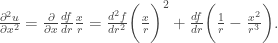
(remember that $r^2=x^2+y^2$ in polar coordinates). Similarly,

$\frac{\partial^2 u}{\partial x^2} = \frac{\partial}{\partial x}\frac{df}{d r} \frac{x}{r} = \frac{d^2 f}{dr^2}\bigg(\frac{x}{r}\bigg)^2 +\frac{df}{dr}\bigg( \frac{1}{r}-\frac{x^2}{r^3}\bigg).$

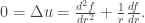
The calculations for the $y$ derivatives are the same as what we have done above, and upon adding them together we find that Laplace’s equation becomes

$0=\Delta u = \frac{d^2f}{dr^2}+\frac{1}{r}\frac{df}{dr}.$

This is an ordinary differential equation! In fact, it is not difficult to verify that

$f(r)= \log r ,$

is a solution to this equation so we by replacing $r^2=x^2+y^2$ we obtain

$u(x,y) = \frac{1}{2}\log (x^2+y^2),$

as a solution of Laplace’s equation! This is the so called fundamental solution of the Laplace equation. Now, in actual applications we would like to solve Laplace’s equation on some subset $\Omega$ of the plane and prescribe the value of the solution on the boundary of this subset so we’re not done with Laplace’s equation just because we found one solution. What is amazing though is that we can ‘build’ these solutions by using the fundamental solution!

To recap, to solve Laplace’s equation we first assume our solution is slightly boring to find a solution. We can then we can use this as a stepping stone to find more interesting solutions. And the way we solve for the initial function is by applying a change of variables!

Summary

So there are two examples (three if you include my motivating example) of how a change of variables can make your mathematical life a little easier. Of course, there are many more examples out there. In fact, the more I look out for them in lectures (and in my own solutions) the more examples I seem to notice.